What Is Radiocarbon Dating? Everything About the Method That Decides Between a Murder Case and an Archaeological Find
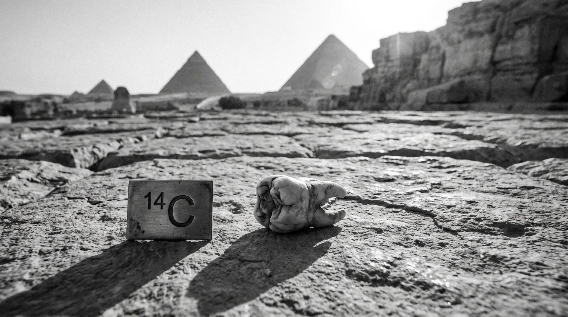

Radiocarbon dating measures how much carbon-14 (C14) is left in a find and determines from that when carbon exchange in the analyzed material ended. How this works mathematically and biologically, how far back it reaches, why a result is never a single calendar year, what a tooth reveals that a bone does not, and where the method breaks down, I explain here using a real laboratory report from my own casework.
There are too many open questions here, and I have been asked them for years without ever answering them in one place. In almost every text I have written about skulls, provenance, seizures ( Is It Legal to Own a Real Human Skull) and the discovery of human remains, the same abbreviation shows up, usually in a subordinate clause, usually as something self-evident. I have never once explained it.
So I sat down over the past few days and put together everything I know about radiocarbon dating, alongside what has been published on it in recent years. What you are reading is an attempt to clear this topic once and for all, from the formation of the isotope high in the atmosphere to that one line on a laboratory report which almost nobody reads and which decides everything.
What is radiocarbon dating?
Radiocarbon dating, also called C14 dating, determines when carbon exchange ended in the biological material under examination. In short-lived material that often corresponds roughly to the moment of death, while in wood, in teeth and in slowly remodeled bone tissue the measured signal can lie considerably earlier. It works because a radioactive carbon isotope forms continuously in the upper atmosphere, carbon-14, which enters every living organism through photosynthesis and the food chain. As long as an organism is alive, it keeps replenishing this isotope and holds its proportion roughly constant. With death the uptake ends, and from that moment the carbon-14 present decays at a rate that no environmental influence accelerates or slows. Measure how much of it remains, and you can calculate backward to when the carbon entered the material and when its exchange ended. How closely that point sits to the death itself is decided by the material.
One confusion has to go right at the start, because I meet it more often than any other. What is meant is always a point on the calendar, the century or millennium in which this organism lived. What is not meant is the age of the individual. Whether this person died at 20 or at 70, a radiocarbon date will not tell you.
The method reaches back roughly 50,000 years. It works on everything that once took part in the carbon cycle, so on bone, teeth, wood, charcoal, leather, textiles, parchment and plant remains, and it dates neither metal nor stone nor the mineral fraction of a ceramic, though it does date suitable organic residues on or in them. And it delivers, and this is the most widely misunderstood point of all, not a single date but one or several time spans, each with its own probability.
What does a radiocarbon date actually tell me?
Picture a skull turned up by construction work. It looks old, but almost every skull looks old once the soft tissue is gone. A person who died in 1985 and a person who died in 3000 BC sit disturbingly close in visual terms once decomposition has run its course. The first police question is therefore not who this was, but whether it is their business at all.
That is precisely the question radiocarbon dating answers, and better than any assessment by appearance. It tells you whether the find dates from the last few decades or lay in the ground for centuries or millennia. A suspicion becomes a time span, and a time span becomes a jurisdiction.
Equally important is what it does not tell you, because that is where most misunderstandings begin. It gives no name and no identity, and for that you need DNA or dental comparison. It gives you no cause of death and does not answer whether a crime occurred at all. And above all it does not give you this person’s age. It answers when he lived, not how old he became in the process. Age at death we read from the skeleton itself ( The Skeleton Does Not Lie), from dental wear, suture closure and bone structure, an entirely different procedure with entirely different margins of error. It gives you no day and no month, only one or several probability ranges. How wide those turn out depends on the age of the sample, on the measurement uncertainty and above all on the shape of the calibration curve at that particular point. For someone who died in the 1970s, bomb pulse dating can become accurate to within a few years, while an unfavorable stretch of curve can span several centuries for a far older find.
And strictly speaking it does not date the human being, but the piece of material that ended up in the laboratory. Which tissue you send in therefore decides which section of a life you are measuring at all. That sounds like a small matter, and it is the most important sentence in this entire text.
That is the thesis that carries this whole piece. A radiocarbon result is not a calendar year. It is a probability distribution, and anyone who reads it as a year has not understood the method, no matter how expensive the instrument was that produced it.
One factual clarification belongs at the beginning, because it prevents a misunderstanding. I do not operate an accelerator, nobody can afford one without a university institute behind them, and why that is so you will see further down in figures. Commissioning, sample selection and evaluation are my part ( radiocarbon dating service), the measuring happens in the laboratory. That sounds like very little, and it is the part where most datings fail.
I consider radiocarbon dating one of the most interesting procedures that archaeology, forensic science and anthropology share. And in my experience one of the most rarely used. I will come back to that point at the end, because it irritates me more than anything else about this subject.
Let us start with the misconception I encounter most often.
No, the method did not wait for the bomb
One notion persists stubbornly, and it runs roughly like this: because atmospheric nuclear testing in the 1950s sent the carbon-14 content of the air shooting upward, and because this so-called bomb pulse is used for dating, radiocarbon dating supposedly only works from that point onward. Everything before that is guesswork, interpretation, reading tea leaves.
That is nonsense on a scale one rarely gets to clear away so cleanly.
Willard Libby and his colleagues Ernest Anderson and James Arnold published the method in Science in a paper on the worldwide assay of natural radiocarbon, and they did so in the year 1949. The first Soviet nuclear test took place that same year, and the large series of atmospheric tests that produced the bomb pulse did not begin until the early 1950s. Libby received the Nobel Prize in Chemistry in 1960 for a procedure that had by then rewritten archaeological chronologies for a decade. The method was finished before the bomb pulse even existed.
The bomb pulse is an additional and entirely independent application, born of a side effect of nuclear testing, and it answers a completely different question than classical dating. Classical dating asks when carbon exchange in a material ended. The bomb pulse asks something else first, namely when this tissue was formed, and in the case of tooth enamel the year of birth can be calculated backward from that through the known sequence of dental development. Both use the same isotope and almost nothing else in common.
How far the classical method reaches back I will say straight away, for the order of magnitude. Roughly 50,000 years, in individual cases with extremely elaborate sample preparation somewhat more. That reaches far beyond the last glacial maximum and thus into a period when Neanderthals still lived in Europe. Anyone claiming this only works since 1963 is confusing an add-on application with the method itself.
Otto Sapiens, that variety of Homo sapiens who knows everything because he once listened to an audiobook about it, will object at this point that none of this can be verified. It can be verified perfectly well, that is what the section on calibration is about, and the verification is called tree rings.
The find where everything begins
Before I go into the physics, I want to show you the question I actually need this method for, because it is more mundane and more urgent than most people assume.
A forest, somewhere in a range of low mountains. A walker who looks down into a hollow off the path. A partly skeletonized body, soft tissue only in remnants, but the lower half still inside a pair of jeans. The police arrive, the prosecutor arrives, and one question stands in the room before anyone thinks about perpetrator, motive or time of the offense: is this a case for the homicide squad or for the state heritage office?
The jeans help less than you might think. Riveted denim has been in circulation for more than 100 years, and cotton denim can survive surprisingly long under certain soil and moisture conditions. A garment does not date the wearer, at best it dates the earliest possible point in time. Anyone who infers a year of death from a pair of jeans has a lead and not a finding.
The boundary that decides whether prosecution is possible at all lies with the statutes of limitations, and those differ from one legal system to the next. In Germany murder never becomes time-barred, which is governed by Section 78 subsection 2 of the Criminal Code, under which crimes covered by Section 211 do not expire. Prosecution of crimes under the German Code of Crimes Against International Law likewise does not expire, under its Section 5. That statute came into force on June 30, 2002, and how offenses committed earlier are to be handled depends on the law applicable to them. In the French cases I am about to cite, by contrast, the authors’ legal assessment depended on the limitation rules in force there. For practical investigative work, the prospect of living suspects, of witnesses, of contemporaneous missing person reports and of directly comparable material nonetheless drops off sharply as the time gap grows. A great age does not, however, automatically turn a find into a purely archaeological matter. There are war graves, historical identifications, colonial acquisition contexts, repatriation claims and unexplained grave disturbances. What dating achieves is therefore not a sorting into important and unimportant, but a clarification of which jurisdiction and which line of inquiry applies at all. And it achieves that more reliably than any assessment by appearance.
The 3 published cases that Benoit Bertrand and colleagues described in 2024 in Forensic Sciences Research show the full range of this decision. In the first case, a partial skull from the beach at Audresselles in northern France, without any context and without an identity, 3 combined measurements produced 2 separate ranges at 95.4 percent total probability, namely 4332 to 4231 BC at 83.9 percent and 4194 to 4168 BC at 11.5 percent. Neolithic, archaeologically significant, and without bearing on the question of a modern homicide. And even this case shows how quickly a distribution turns into a single number, because the abstract of that same paper cites one calibrated age of 4232 BC. In the second case, skeletal remains from the flooded underground of a historic fort near Wimereux, the carbon content lay well above the modern reference value. Combined bomb pulse calibration produced for the bone tissue examined an initial range of 1962 to 1963 at 14.2 percent or 1974 to 1976 at 81.3 percent probability. In France crimes become time-barred after 20 years, with exceptions that include war crimes, and crimes against humanity do not become time-barred there at all. Under that assessment the case fell outside the relevant period. The sample came from cortical femoral bone, and for that the authors give a lag between the actual and the measured year of death of 29.5 years in the median and 32.0 years in the mean, which pushes the finding dangerously close to the limitation boundary. The third case is the most interesting, and I will come back to it in detail later, because it proves what laypeople and unfortunately some investigators too get wrong on a regular basis.
How the forest case ended I will not write here. That is not my decision and not my proceeding. What I can write is the path by which one arrives at the answer, and I will now walk that path from the beginning.
A nitrogen atom is struck by a neutron
High in the atmosphere, in the stratosphere and upper troposphere, cosmic radiation hammers down on the air envelope without pause. It produces secondary neutrons in collisions, free neutrons that fly through the thin air and eventually strike an atomic nucleus. When such a neutron hits a nitrogen-14 nucleus, and this gas is by far the most abundant constituent of our atmosphere at roughly 78 percent, something elegant happens: the neutron is captured, a proton is knocked out, and what remains is carbon-14.
The nucleus afterward has the same mass number but one proton fewer and one neutron more, so it is no longer nitrogen but carbon, an unstable one. This newly formed carbon-14 behaves chemically much like the stable carbon isotopes, but it is subject to small isotope-dependent fractionation effects. It oxidizes to carbon dioxide, mixes into the atmospheric carbon pool, and from there every plant takes it up through photosynthesis, unable to tell whether it is building in a stable or a radioactive atom.
What the plant takes from the air and builds into biomass passes through herbivores and further food chains into animals and into human beings. Every living organism is therefore in permanent exchange with the atmospheric carbon reservoir, and the isotope ratio in its tissue follows the reservoir it actually draws on. In terrestrial food chains that reservoir usually sits close to the atmospheric signal, while marine, freshwater and geologically influenced systems can deviate considerably.
How rare this isotope is deserves a moment, because it explains where the real technical achievement lies. For roughly one trillion carbon atoms in the natural atmosphere there is about a single carbon-14 atom. A trillion is a 1 followed by 12 zeros. If you could check one carbon atom every second, without pause and without sleep, you would be busy for well over 30,000 years before the first C14 turned up. That is the needle in the haystack the machines I describe further down are counting, and they count them one at a time.
The clock starts running when the exchange stops
As long as an organism lives, the decaying C14 is permanently replenished, because it goes on breathing, eating and rebuilding tissue. The proportion in its tissue therefore stays roughly constant and follows the value of its surroundings.
With death this exchange ends abruptly. From then nothing is replenished, and the carbon-14 present decays on, in a process no environmental influence accelerates or slows. Through beta decay it converts back into nitrogen-14, the very thing it came from. The circle closes, and what remains is a clock. For the organism as a whole, further carbon uptake ends with death, but the clock measured in the laboratory for a particular tissue may have stopped considerably earlier, for instance with the formation of tooth enamel, or it may integrate a long period before death because of slow remodeling.
The mathematical core is a one-liner, and I write it out because it is simpler than its reputation. The number of remaining atoms equals the original number multiplied by e to the power of minus lambda times t. Lambda is the decay constant, t the elapsed time. Solve that for t and you have the age. If you want to express the decay constant through the half-life, divide the natural logarithm of 2 by the half-life, and with that the entire basic mathematics of the method has been told.
The rest are corrections, and the corrections are the reason a radiocarbon report runs to 2 pages rather than 2 lines.
One of those corrections concerns fractionation. Plants prefer lighter carbon isotopes during photosynthesis, and depending on metabolic pathway they do so to differing degrees. A C4 plant such as maize or millet fractionates differently from a typical C3 plant such as wheat or a central European tree, and a marine animal differently from both. Without correction the same elapsed span would yield different ages in different organisms, a noticeable drawback for a method meant to measure time. Every radiocarbon age is therefore normalized through the measured ratio of carbon-13 to carbon-12 to a standard value, and that standard value is minus 25 per mil. When you find a line on a certificate labeled delta-13C, this is its purpose, before it tells you anything at all about diet.
Why we calculate with a half-life everyone knows is wrong
Now it gets briefly curious, and I like this passage because it shows how science handles its own errors once it has grown up.
Libby determined the half-life of carbon-14 as 5568 years. That was the best available measurement of its day, and the entire early radiocarbon literature calculated with it. In the early 1960s more precise measurements put the true value at about 5730 years, with an uncertainty of roughly 40 years. Harry Godwin published that in Nature in 1962, and since then this figure has been known as the Cambridge half-life, while the old value remained the Libby half-life.
And now comes the part where laypeople regularly get off the train: laboratories still calculate with the wrong number to this day, deliberately and worldwide.
That is not sloppiness but a conscious convention, laid down by Minze Stuiver and Henry Polach in Radiocarbon in 1977. The reason is as simple as it is compelling. The conventional radiocarbon age is no statement about the true calendar age but a standardized intermediate quantity that has to be calibrated anyway. As long as everyone calculates with the same value and the calibration takes that value into account, the half-life cancels out of the result again. Had the field switched in the 1960s, every date published earlier would have become incompatible, and every archaeological chronology would have needed a conversion factor in mind.
Anyone who does want to convert divides the age calculated with 5730 by 1.029, and there is nothing more to this conversion than that.
Belonging to the same family of conventions is the abbreviation BP, which you will find on every report. It stands for „before present”, and the present is fixed at the year 1950. The reason for that is twofold. First, the calibration datasets refer to it, and second, 1950 lies before the massive change in atmospheric C14 content caused by the thermonuclear test series of the following years. The modern activity itself is not defined through some arbitrary piece of old wood, but through internationally agreed oxalic acid standards and a mathematically fixed normalization.
This leads to a formulation I never write down without a quiet pleasure. When a report states 2517 BP, that means 2517 years before 1950, and all of you reading this were, by the counting convention of radiocarbon dating, born in the future. A convention that has outlived its own justification by more than 70 years and is kept anyway, because switching would do more damage than the error it holds. I know public authorities that cling to far worse rules for far worse reasons, only without the self-irony of printing it on every form.
The core remains: BP is not a calendar year in the everyday sense but a computational quantity, and anyone who confuses it with a calendar date is off by decades to centuries.
The limit at 50,000 years, and why 1 percent of dirt tears it down
Why does it stop at roughly 50,000 years? After 10 half-lives, less than 0.1 percent of the original quantity remains. The sample then holds so few C14 atoms that counting statistics collapse and the instrument background grows larger than the signal. At that point you are no longer measuring the sample but the machine.
The real killer, however, is not the residual activity but contamination, and here sits a number you should commit to memory, because it explains all the care that goes into sample preparation.
Take a sample that is infinitely old, holding no C14 of its own at all. Contaminate it with 1 percent modern carbon, through a fine root, through humic acids from the soil, through hand sweat, through a conservation agent. That sample then measures out at roughly 37,000 years. A result that looks like a serious finding, with a handsome uncertainty beside it, consisting entirely of dirt somebody failed to remove. A sample with a true age of 40,000 years slips under the same contamination to roughly 33,000 years.
A single percent, one hundredth of the material, decides here over more than 7,000 years.
That is why every proper finding must state which preparation procedure was used, and why a result without traceably documented preparation carries no forensic weight. Whether that appears on the certificate itself or in the supplementary laboratory records is secondary, but it has to be findable. On the report I am about to show you it says acid-base-acid treatment and collagen extraction, and those 2 lines matter more than half of the rest.
At the young end sits a mirror-image problem. Material from the decades before the nuclear tests is barely distinguishable from the modern reference value, because the differences lie within the measurement uncertainty. This is aggravated by the Suess effect, named after Hans Suess: since industrialization we have been blowing enormous quantities of fossil carbon into the air, coal and petroleum so old that all of their C14 decayed long ago. That carbon dilutes the atmosphere and makes it age in radiocarbon terms. A tree growing today therefore looks older than it is.
In practice this means that between roughly 1650 and 1950 the resolution becomes poor. A skeleton from that span can be placed approximately, but separating 1850 cleanly from 1920 is usually beyond radiocarbon alone.
A radiocarbon year is not a calendar year
And with that we arrive at the point where most misunderstandings arise.
The whole calculation above tacitly assumes the C14 content of the atmosphere was always the same, and it was not. The cosmic radiation that produces C14 is modulated by the Earth’s magnetic field and the solar wind, and both fluctuate. The magnetic field changes strength over millennia, solar activity over decades to centuries, and ocean circulation shifts how much carbon is exchanged between air and water at any given time. The atmospheric starting value was therefore a moving target across the millennia.
So the measurement first yields only a conventional radiocarbon age, and that age has to be translated into calendar years through a calibration curve.
This curve rests on extensive, independently dated measurement series. It is not, however, a mere stringing together of those series but a statistically constructed model of that data, with declared uncertainties and modeled transitions between the datasets. How this model is built was described by Timothy Heaton and colleagues in a methods paper of its own, whose very title names the procedure outright, Bayesian splines with errors in variables. Anyone selling the curve as a pure measurement series is suppressing that very layer. It rests on material whose calendar age is independently known and whose C14 content is simply measured out. The most important supplier is tree rings. A tree forms one ring per year, and overlapping ring sequences of living and dead timber build unbroken chronologies across many millennia. For every single ring one knows exactly in which calendar year it grew, and one then measures how much C14 the tree built in that year. For the oldest sections, annual layers in lake sediments, corals, speleothems and foraminifera from marine sediments are added.
The current curves were published in 2020. IntCal20 for the Northern Hemisphere, produced by Reimer and colleagues, SHCal20 for the Southern Hemisphere under the lead of Hogg, and Marine20 for marine material, developed by the group around Heaton. That the hemispheres are treated separately has a measurable reason: Hogg and colleagues put the mean Southern Hemisphere offset at 36 plus minus 27 radiocarbon years, so material from there appears older on average. All 3 reach from the present back to 55,000 calendar years. Anyone calling calibration arbitrary has before him a curve built from tens of thousands of measurements on independently dated material, cross-checked by competing groups in several countries.
Now comes the decisive effect. This curve is not smooth. It has bumps, dips and, most awkwardly, plateaus. A plateau is a stretch where the curve runs almost horizontally, so several different calendar years produce the same C14 value. If your measurement hits such a plateau, you get no sharp result but a broad one, and frequently a multimodal one.
The most famous of these plateaus lies between roughly 800 and 400 BC and is called the Hallstatt plateau. It is the reason the European Iron Age is chronologically so intractable, and it is the reason the certificate I am about to show you gives 3 answers instead of one.
That is not a measurement error and not a bad sample, but the result of atmospheric C14 fluctuations at the time, driven among other things by solar activity, the Earth’s magnetic field and the carbon cycle.
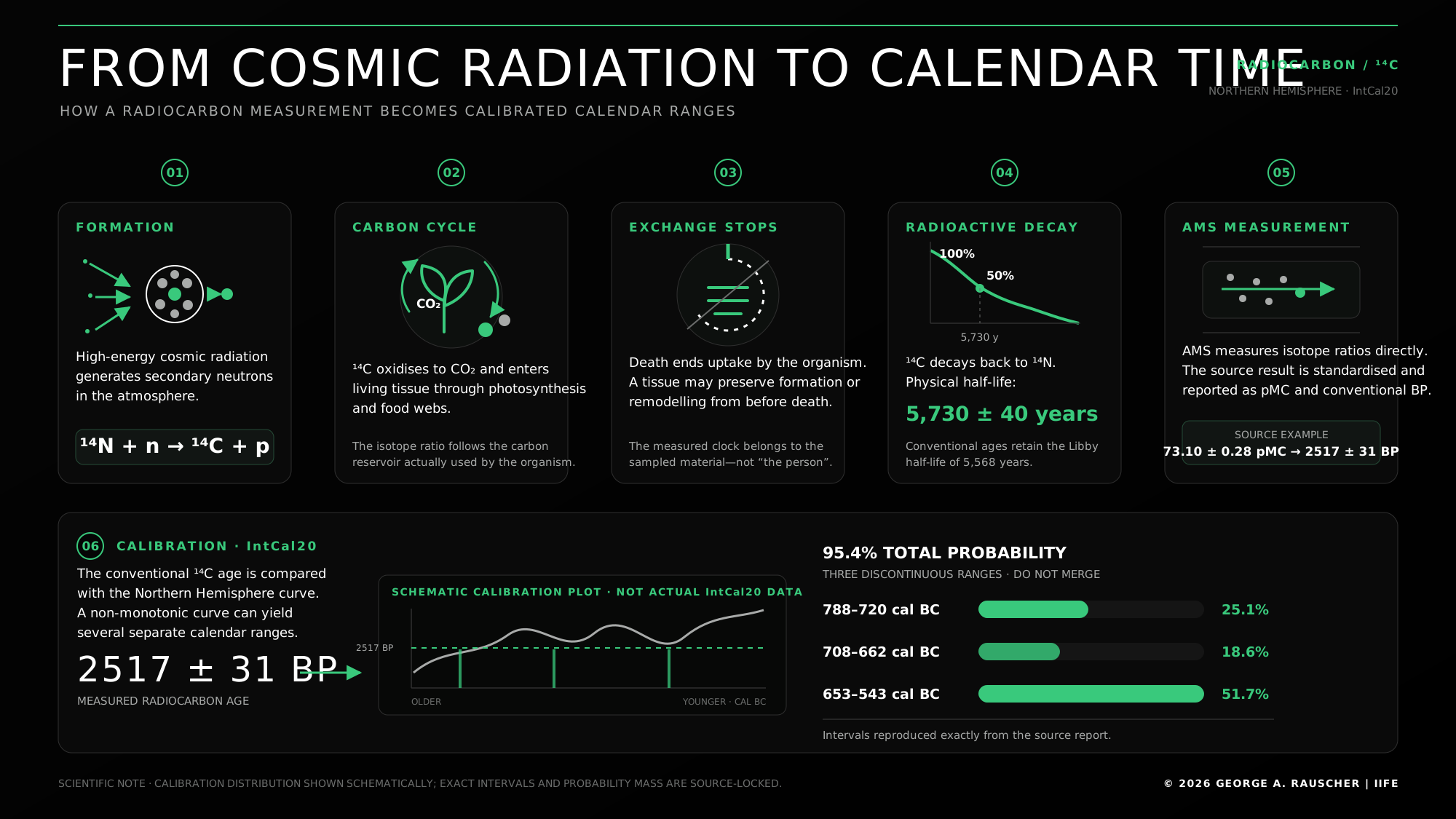
High-energy cosmic radiation generates secondary neutrons that convert nitrogen-14 into carbon-14. After carbon enters living tissue and exchange eventually ends, AMS measures the isotope ratio and produces a conventional radiocarbon age. Calibration against IntCal20 converts the result into three separate calendar ranges totalling 95.4% probability. The calibration plot is schematic; all reported intervals and probabilities reproduce the source report exactly.
The certificate, line by line
For this I am using a real report from my own casework ( IIFE C14 Analysis Report). The sample designation reads „Female mummy 215, Thebes 1877″, the material is a tooth, specifically a maxillary molar. I say no more about its provenance, because clients and procedural details do not belong on my blog. The results I show in full, because from them you can learn how such a document is read.
If you want to see who this is actually about, the photograph of this mummy and the radiographs appear in an older article on this site, which approaches the subject more popularly than this one does.
The first line that counts is the radiocarbon age: 2517 plus minus 31 BP.
The 2517 are radiocarbon years before 1950, calculated with the Libby half-life and corrected for fractionation. The 31 is the standard deviation, or 1 sigma. Roughly speaking that means a probability of about 68 percent that the true conventional value lies between 2486 and 2548. It does not mean that anything about this sample is exactly 2517 years old.
The second line is the pMC value: 73.10 plus minus 0.28. pMC stands for „percent Modern Carbon”, the percentage share of the modern reference carbon. 73.10 pMC means that the sample shows 73.10 percent of the normalized modern reference activity. That is not the same as saying that exactly 26.90 percent of its individual original inventory has decayed, because nobody knows that starting inventory. What the instrument measured are isotope ratios, and the pMC value is the central result quantity calculated from them, from which in turn the conventional radiocarbon age is derived, using a formula that is printed out on the report itself: t equals minus 8033 times the natural logarithm of pMC divided by 100. Enter 73.10 and you get 2517.1, which rounds to exactly the number in the first line. Enter the uncertainty, that is 8033 times 0.28 divided by 73.10, and you get 30.8, which rounds to the 31. You can check this certificate with a pocket calculator. With the rounded values the stated age has to be reproducible to a close approximation, and any relevant deviation belongs discussed with the laboratory before the finding gets cited anywhere. Hidden inside that constant 8033, incidentally, sits the entire convention from the previous section, because 8033 times the natural logarithm of 2 gives 5568, which is precisely the Libby half-life. Anyone who takes the formula on his report seriously can work the half-life used back out of it, without its ever being written down. For forensic practice, remember a rule of thumb that will serve you better than any formula: a value below 100 on its own proves no formation date before 1950, because fossil carbon, reservoir effects and the meanwhile falling atmospheric values push it downward as well. If, on suitable terrestrial material, it lies clearly above 100, and with this isotope that is possible, then the sample contains bomb carbon, and the tissue examined was formed after the start of atmospheric nuclear testing. Whether a birth range, a death range or merely a tissue range integrated over years follows from that is decided solely by the choice of material. A glance at a single number nonetheless separates the orders of magnitude straight away.
Then come the 2 stable isotope values. Delta-13C comes in at minus 19.06 per mil, delta-15N at 11.95 per mil. Only the carbon value has a technical function in the age calculation, where it serves the fractionation correction. The nitrogen value does not enter the C14 calculation at all, it is an independent parameter for diet and environmental conditions. Beyond that they tell us something about diet, and I write more about that further down, among other reasons because I very nearly fooled myself at this exact point.
Next come preparation and reference materials, specifically an acid-base-acid treatment with subsequent collagen extraction. The standards used were NIST-OXII and phthalic anhydride. NIST-OXII serves as the modern reference standard. The phthalic anhydride is fossil, practically C14-free material against which the process and instrument background is monitored, the question of how much foreign carbon one’s own workflow drags in. This background correction has to be traceably documented within a laboratory’s quality management, even if not every raw value appears on every customer certificate.
Measurement was performed by accelerator mass spectrometry with automated sample graphitization at an accredited laboratory. Calibration was carried out with OxCal version 4.4.4, the software by Christopher Bronk Ramsey that counts as the standard tool in the radiocarbon world, against the curve by Reimer and colleagues from 2020, that is IntCal20, in the variant for the Northern Hemisphere atmosphere. The command itself appears on the report and reads R_Date with the parameters Sample A, 2517 and 31. The plot header additionally carries the entry r:5, and that one is a small minefield of misunderstanding. It does not mean revision 5 but a bin width of 5 years for the calculated probability distribution. Anyone concluding from this that all interval boundaries must be divisible by 5 is mistaken, because OxCal by default does not round the ranges at all, and its reference point does not sit at 1950 but at the middle of the year 1950. Finally, it is explicitly noted that neither a Bayesian sequence model nor a reservoir correction nor a regional delta-R offset was applied. That line about what was NOT calculated is forensically worth more than most lines that assert something, because it tells you which assumptions were left open.
And the outcome of this calibration is the reason I chose this particular report.
At 68.3 percent probability there are 3 intervals: 774 to 749 BC at 15.5 percent, 687 to 666 BC at 12.5 percent, and 641 to 569 BC at 40.3 percent. At 95.4 percent probability there are likewise 3 intervals: 788 to 720 at 25.1 percent, 708 to 662 at 18.6 percent, and 653 to 543 at 51.7 percent.
There stands a machine worth a single-family house in a good neighborhood, it counts individual atoms out of a trillion, it achieves a measurement precision of under half a percent, and then it hands you 3 separate time windows for a single tooth, scattered between 788 and 543 BC. And the report adds that these 3 ranges are components of one single probability distribution and must not be merged into a continuous interval. Anyone turning 788 to 543 into one span has invented a single statement out of 3. Anyone taking this for a failure of the method has not understood how the calibration curve is built, because it is the exact opposite. It is the only honest answer available, because each of these 3 windows is compatible with the measured radiocarbon value once the measurement uncertainty and the uncertainty of the calibration curve are taken into account. The multimodality arises, as the report puts it, because the measurement likelihood together with the uncertainty of the curve maps onto a non-monotonic stretch of IntCal20, a place where the curve does not run obediently in one direction but swings back on itself. A laboratory that turns this into a single calendar year for you has not measured better, it has reduced a multimodal probability distribution to a misleading point value.
We are sitting here in the older part of the Hallstatt plateau, in the very zone where the calibration curve swings back on itself repeatedly. The 51.7 percent for the youngest window is the most probable single range, but it is not certainty, it is a narrow majority.
Three clocks in a single human being
Now comes the part I consider the most important of this entire text, and it is also the part I most often have to explain in practice, usually to people who ought to know already.
A human being is not a uniform object. He is a bundle of tissues formed at completely different times and renewed at completely different rates. When you take a sample, you are not taking „the human being” but one specific window of time out of his life. Which one, you decide through the choice of tissue, and that decision is made before the laboratory, not after it.
Douglas Ubelaker condensed this logic into the standard review in the Journal of Forensic Sciences in 2014, and it begins with the most stable tissue. Tooth enamel is the steadiest clock in the whole body. It mineralizes in childhood and adolescence, in a sequence that falls earlier or later by tooth position and for which the London Atlas by Sakher AlQahtani and colleagues is the customary reference, and after that nothing more happens. No biological remodeling, no relevant carbon turnover, no regrowth. Anyone who loses tooth enamel as an adult does not get new enamel. What is a disadvantage biologically is a gift forensically, because this enamel preserves the atmospheric signal of those childhood years unchanged until decomposition and far beyond it. That is what determination of the year of birth through the bomb pulse rests on ( When Teeth Speak).
The dentine beneath behaves differently. Primary dentine forms together with crown and root, after which the tooth slowly deposits secondary dentine for life. A bulk dentine sample can therefore predominantly reflect the tooth formation phase, depending on which region was sampled, but it can also contain appreciable later fractions, and which section was taken has a hand in deciding that.
Bone is the most restless of these clocks. Bone is permanently remodeled, broken down and rebuilt, and its collagen is therefore a moving average across years. Robert Hedges and colleagues modeled this at the femoral mid-shaft in the American Journal of Physical Anthropology in 2007, in 67 individuals who died in Australia between 1990 and 1993 at ages between 40 and 97, and they used the bomb pulse itself as their marker. The result: in women the turnover rate falls from about 4 percent per year at 20 to about 3 percent at 80, in men it runs 1.5 to 3 percent over the same span, and during the growth phase between 10 and 15 it shoots up to 5 to 15 percent.
The sentence from that paper I consider the most consequential says, in substance, that human femoral collagen reflects an individual’s diet over a considerably longer period than 10 years, including a substantial share of collagen already formed during adolescence. A femur is therefore not a window onto the last years even of an 80 year old, but still carries material from the time when he learned to ride a bicycle.
Trabecula-rich regions such as ribs, vertebrae and parts of the pelvis turn over faster on average than the compact femoral shaft, because they offer more surface per volume. Douglas Ubelaker, Bruce Buchholz and John Stewart made a trick out of that in 2006 which I consider one of the most elegant in the whole discipline. Because trabecular bone remodels faster, its radiocarbon values for formation before 1963 lie higher than those of cortical bone from the same skeleton, and for formation after 1963 the relationship reverses. Comparing trabecular and cortical bone from the same deceased individual can therefore give an additional indication of which side of the bomb peak you are standing on. They demonstrated this on 2 individuals with known years of birth in 1925 and 1926 and known years of death in 1995 and 1959. That is an elegant proof of concept and not a decision rule that carries on its own, because turnover rates vary considerably between individuals and between anatomical sites. Their collagen does not become point-accurate either, there too it remains a signal integrated over years, and the rates fluctuate substantially with person, age, sex and disease. Soft tissue renews itself within months. Scalp hair grows on average about 1 centimeter per month and can be measured segment by segment, so that a long strand yields a rough sequence of the final months of life. A clock it is not, because individual growth rates and hair cycles shift the assignment. And the crystallins in the nucleus of the eye lens form, as Niels Lynnerup and colleagues showed in PLoS ONE in 2008, almost entirely around the time of birth. After that there is only a very small and further declining new formation, while crystallins once formed undergo practically no turnover. With a suitable formation model the year of birth can be estimated from them.
How far apart this drifts in practice is shown by the third case from the paper by Bertrand and colleagues that I announced above. A skeleton near Valenciennes, with a suspected identity. Different tissues from the same person were dated. The bone sample produced a calibrated tissue range between 1998 and 2002 at 84.6 percent probability. The hair sample produced 2013 to 2018 at 83.3 percent. In raw terms that leaves roughly 15 years between them, on one and the same body, with one and the same method, in the same laboratory. The authors name the reason outright, the slower remodeling of bone tissue, and they compute it out. For trabecular vertebral bone they apply a mean lag of 8 years following Ubelaker and thereby arrive at 2006 to 2010, at which point the 2 findings converge markedly. DNA analysis subsequently confirmed the identity of a person who had been reported missing a decade before the discovery, and the teeth supplied the matching year of birth.
Anyone who had dated only the bone in this case would have placed the year of death more than a decade too early and would have searched the wrong period in missing person databases, not because of a measurement error but because of the choice of tissue.
What that means for my molar
And with that back to my certificate, because there is one word on it from which everything hangs: collagen extraction.
Collagen does not sit in the enamel of a tooth. Enamel is more than 95 percent inorganic mineral, with practically no collagen. The collagen sits in the organic dental tissues, above all in the dentine and in the cementum of the root. From the entry collagen extraction it therefore follows with certainty that no enamel carbonate was measured, and that already makes 2 different materials within the same tooth with 2 different time windows.
What does not follow from it, and at this point I have to correct myself, is the claim that it was pure dentine collagen. Cementum contains collagen as well, and it goes on being deposited into adulthood. Andrea Czermak and colleagues warned about this very point in 2020: anyone sectioning a tooth horizontally into halves or quarters risks mixing growth layers and including unwanted cementum or secondary dentine. Their counterproposal is micro-sampling at anatomically defined positions that avoids those zones.
Whether in my sample dentine alone was extracted or a mixed organic dental fraction is decided by the mechanical preparation before extraction, and that does not appear on my certificate. Without that information I am not entitled to speak of dentine collagen. Bertrand and colleagues describe this same problem in their third case: because they needed enough material, they took a generous tooth sample spanning several tissues, which enlarged the lag and lowered the accuracy. To get the year of birth sharp, one would have had to sample enamel or primary dentine at a precisely defined location.
From this follows a statement the report itself records in its section on forensic limitations, namely that this age need not be identical to the person’s date of death, depending on the dental tissue sampled and on its formation and remodeling history. In plain terms: the 2517 plus minus 31 BP do not date the death of this woman directly. They reflect the formation period of the organic dental fraction that was actually extracted. If the sample contained predominantly primary dentine, the center of gravity probably lies in childhood and adolescence. If secondary dentine or cementum was included as well, considerably later fractions from adult life may have entered it.
If this woman died at 40, the center of gravity of the measured signal can lie years to decades before her year of death, depending on the tooth and on the dentine region sampled. In a sample from the first millennium BC this offset largely disappears into the scatter of the calibrated intervals, spread across more than 2 centuries in any case. It disappears not because it does not exist, however, but because the noise is larger than the signal. And it is systematic, it always points in the same direction, namely too old.
In a modern case the same offset would be devastating. Anyone who dates the tooth in a forest case and writes the result into an expert report as the year of death hands the prosecutor a number that can be off by half a lifetime. That is why the question of which tissue to send in is not a logistical question but the central technical decision of the entire procedure.
There is a second consequence that hardly anyone thinks through. If the sample contained predominantly early-formed dentine, then the isotope values on this report do not describe this woman’s diet as an adult either. They very probably describe the diet during tooth formation for the most part, though depending on the composition of the sample they may contain later fractions as well. Anyone inferring her social standing in adult life from minus 19.06 and 11.95 per mil is reading the wrong phase of life and does not even know it.
A rib or another trabecula-rich bone would on average have reflected a later life window than compact femoral shaft. Its collagen would not have dated the death point-accurately either, but again a period integrated across years. That is the real conflict of objectives: the tissue with the most precise time reference is rarely also the one with the best preservation. Teeth often win this conflict because they survive exceptionally well, but you pay for that with a time window that can lie long before death.
The Nile fish I very nearly invented
Now the passage where I have to correct myself, and I write it out because you should see how such an error comes about and how it gets stopped.
The nitrogen value on my report is 11.95 per mil, and that is a high value. The standard interpretation of elevated delta-15N reads: higher trophic level, so more animal protein, and with a share of freshwater fish the value rises particularly sharply. In a woman from Thebes, a city directly on the Nile, the inference that she ate a lot of fish lies close at hand.
And if she had eaten a lot of Nile fish, we would have a problem. Because fresh water flowing through limestone carries dissolved carbonate carbon from geologically old rock holding no C14. Water plants build this old carbon in, fish eat the water plants, humans eat the fish, and at the end a person who never did anything wrong measures out centuries too old. This is called the freshwater reservoir effect, and the Nile catchment has limestone in abundance. A study of freshwater shells from the Nile was later interpreted as an indication of a reservoir offset of roughly 500 radiocarbon years.
I had the passage finished in my head. Elevated delta-15N, Nile fish, reservoir effect, date possibly several hundred years too old, an elegant arc from the isotope line to the dating line on the same sheet of paper.
Then I checked the literature, as I do with every claim before it goes into a text. And the literature took my passage apart.
Alexandra Touzeau and 8 colleagues examined this very question in the Journal of Archaeological Science in 2014, on Egyptian mummies from a span of 5,500 to 1,500 years before present, on hard and soft tissues, with carbon, nitrogen and additionally sulfur. Their finding on my point is unambiguous. First: Touzeau and colleagues interpret the high delta-15N values of the Egyptian population they studied primarily as an aridity signal and not as evidence of a particularly high share of animal protein. In extremely dry ecosystems the nitrogen values in soils and plants shift upward, and that signal travels through the entire food chain without anyone having eaten more meat or more fish. Second, and this is the actual proof: in the population studied by Touzeau and colleagues the sulfur isotopes argued against regular consumption of fish such as Nile perch. For my woman from Thebes that is a statement about her time and her region, but not a finding about her personally, because a sulfur value of her own is precisely what is missing. Third, the diet was almost exclusively C3-based, the C4 share lay below 10 percent, and the origin of the food was, according to earlier strontium data, confined to the Nile valley.
So my beautiful passage was wrong. Not narrowly off, but reversed in its causal chain.
What occupies me about it is not the error itself but how plausible it felt. Elevated nitrogen, a river at the doorstep, a well-known reservoir effect, everything fits together. This is how false expert reports come about. Not through carelessness, but through a chain that looks reasonable at every single link and still comes out at the wrong end, because one link was never checked. I have seen this in proceedings where more was at stake than a woman who died 2,600 years ago.
And there is a further lesson that is more practical. Had I also commissioned sulfur, delta-34S, at the time, and had I possessed local comparative values, the question could have been narrowed down considerably better. Sulfur alone would not have been proof for or against fish consumption either. On my sample it is missing, and so for this one woman the answer stays open. The report itself puts it strictly at this point and states that the reported carbon and nitrogen values alone can neither exclude nor quantify a dietary reservoir effect, because that would require local isotopic baselines, dietary context and where applicable a suitable mixed-source calibration model. That is not a satisfying sentence, but it is the honest one.
The freshwater reservoir effect itself remains real nonetheless, and where it strikes, it strikes hard.
Reservoir effects that really bite
The best known is the marine one. The deep sea exchanges carbon with the atmosphere only slowly, so seawater is depleted in C14. Everything living from it appears typically several hundred radiocarbon years older than contemporaneous terrestrial samples. Marine20 models this global and time-varying effect, and regional deviations are accounted for through local correction values. A person who lived predominantly from the sea carries part of this shift in his bones, and the marine share of his diet has to be estimated from the isotopes in order to correct for it.
The freshwater effect is more treacherous, because it turns out completely differently from place to place. Carbonate rock is the most common cause but not the only one, since old organic carbon, groundwater and geothermal carbon sources can produce substantial offsets as well. Bente Philippsen collected the orders of magnitude in a review in 2013, and the number in it should make anyone cautious: within a single river, age differences of up to 2,000 radiocarbon years can occur.
The cleanest example comes from the Stone Age sites at the Iron Gates, that gorge where the Danube breaks through between Serbia and Romania. Gordon Cook and colleagues dated human remains there in Radiocarbon in 2001 alongside artifacts made from the bones of terrestrial ungulates and directly associated with the burials. The human samples appeared roughly 300 to 500 years older than the terrestrial comparison material, which the authors explained through a heavy share of Danube fish in the diet.
Picture that for a moment in an investigative context. Two skeletons in the same pit, the same soil horizon, the same backfill, and the dating sets them 400 years apart. Anyone unaware of this effect constructs from it a history of occupation, a secondary burial, in the worst case a narrative about reinterments that never happened. And he will tell it convincingly, because after all he has numbers.
There are further variants of this effect. In geothermally active regions C14-free carbon dioxide rises from the ground, is taken up by plants and ages everything that lives from them. And there is the old wood effect: a beam can come from the heartwood of an already very old tree, so that the dating gives not the construction year of the house but the growth year of a timber that was long old when it was felled.
What makes a sample younger and what makes it older
Contamination is the second great source of error, and it works in both directions.
Downward, toward younger, works everything that introduces modern carbon, such as fine living roots growing into porous bone, or simply hand sweat during recovery. Humic acids from the surrounding soil do not belong in that drawer, because depending on the origin and age of the soil material they can shift in either direction. Conservation agents, by contrast, belong unambiguously in neither direction, and that is what makes them such a nuisance. Biogenic or young substances such as certain shellacs make a sample younger. Petroleum-based paraffins, acrylates and synthetic resins consist of fossil, practically C14-free carbon and make it older instead. With historical mixtures, often nobody knows anymore which product was even used, and some polymers can only be removed incompletely by chemical means. Historical collection specimens were treated over decades with shellac, polyvinyl acetate, paraffins, glues and resins, partly for stabilization, partly for cosmetic reasons, and almost never with documentation that would still be findable 100 years later.
This is why old anatomical collection skulls are the most thankless samples one can be handed. They look magnificent, they are complete, they often even carry a label, and chemically they are a grab bag. Nobody knows what went on them in the 1890s, nobody knows what was touched up in the 1950s, and nobody knows whether the piece spent time in a workshop where it came into contact with whatever gets used in such places. And yet these are the pieces that proceedings are built on.
Upward, toward older, works old carbon from carbonates. Lime from groundwater that deposits itself into porous material. Hence the acid-base-acid treatment: the first acid dissolves carbonates, the base removes humic acids, and the second acid removes carbon dioxide that reattached itself from the air during the base treatment.
With bone and teeth, collagen extraction is added, usually following the modified Longin method or with additional ultrafiltration. Whether the collagen is then usable is checked against quality indicators, and you should know them if you ever have to assess a certificate. The atomic ratio of carbon to nitrogen has to lie between 2.9 and 3.6, a criterion going back to Michael DeNiro and a paper in Nature from 1985. The carbon share should exceed 13 percent and the nitrogen share 4.8 percent, values that go back to Stanley Ambrose. These are established guide values and not official limits, because every laboratory additionally assesses collagen yield and elemental content against its own validated ranges. Values outside validated ranges point to inadequate preservation, to foreign input or to problematic preparation. They compel either rejection of the sample or a traceable justification with additional quality data.
These indicators do not appear on my report. That is no reproach to the laboratory, because such values may well exist in its quality records, they are simply not assessable from the customer certificate itself. It is, however, the reason I can speak only in a limited way about this woman’s diet on the basis of this report, and the reason I write that down rather than pretending it does not matter.
The machine that costs millions and wears out anyway
How do you count an atom that occurs once in a trillion?
There are 2 routes for that, and the older one is called decay counting. You place the sample in a proportional counter or liquid scintillation counter and wait for atoms to decay, because every decay yields a measurable signal. The drawback is obvious: with a half-life of more than 5,000 years, almost nothing decays per second. You need grams of material and counting times of days to weeks.
The modern route is called accelerator mass spectrometry, AMS for short, and it does not wait for decay but counts the C14 atoms present directly. That reduces the material required by roughly a factor of 1000 and the measuring time to hours. German laboratories give as the lower bound for their standard service an order of magnitude of half a milligram of carbon after chemical pretreatment, with routine measurements on sufficiently large and well preserved younger samples frequently reaching analytical uncertainties of a few decades.
How this works technically is a chain of tricks, and one of them is so elegant that I enjoy explaining it every time.
For the classical measurement with graphite cathodes the sample is first reduced to graphite and pressed into a metal holder, and alongside that there are now gas ion sources as well. This holder is bombarded with cesium in an ion source, which knocks carbon atoms out and charges them negatively in the process. And here lies the trick. The great interference at mass 14 would be nitrogen-14, which after all has practically the same weight and occurs abundantly in every sample. But nitrogen forms no stable negative ion. An N minus ion falls apart immediately. By working exclusively with negative ions, the single most serious interference problem of the entire measurement disappears by itself, without one additional component.
The ions are then accelerated through a stripper, a thin gas or foil in which molecular ions of the same mass are broken up by collisions. What remains are individual atomic nuclei, separated by mass through magnets and counted one at a time. In parallel the instrument measures the ratios of C14 to C12 and of C13 to C12, which is why the fractionation correction falls directly out of the same measurement.
The early installations were monsters. William Kieser and colleagues described the facility at the University of Ottawa in 2015, a custom-built 3 megavolt tandem, roughly 44 tons in weight, about 25 meters long, with setup costs of around 10 million Canadian dollars. Stewart Freeman and colleagues write of the Scottish SUERC that a 3 year Joint Infrastructure Fund award of 3.9 million pounds financed the accelerator, a purpose-built laboratory and staff there, and the facility opened in September 2002. And the National Science Foundation lists in its award schedule for 1998, under application number 9871035, an amount of 1,335,000 dollars to the University of Arizona for the acquisition of a new instrument alone. Commercial laboratories put it more briefly and say that establishing and maintaining such a system costs several million dollars.
What these figures do not show is the running of it, and for that there is one piece of evidence I value highly because it is unusually candid. Ravi Prasad and colleagues from the Center for Applied Isotope Studies at the University of Georgia described in Radiocarbon in 2013 why their institute acquired a second accelerator. After a decade of operation, failures from worn components inside the accelerator tank were piling up. In the 2 years before that alone, the charging chain, the generating voltmeter, the bearings of the chain motor, the shaft motor and the sheaves of the charging pulleys all had to be replaced. An instrument worth millions, and what brings it down are bearings and pulley sheaves, exactly the sort of part that also fails on a lawn mower.
That is what the current generation of instruments answers. The MICADAS was developed by Hans-Arno Synal and colleagues at ETH Zurich and is marketed commercially today. At 3.2 by 2.6 by 2 meters it is barely larger than a compact car, and it works at 200 kilovolts instead of megavolts. That voltage is supplied by a solid-state power supply without moving parts, the terminal is vacuum insulated, and for that reason the system needs no sulfur hexafluoride as an insulating gas. The helium stripper reaches up to 47 percent transmission, the sample changer holds 40 cathodes, precision reaches 0.2 percent or better, blanks beyond 50,000 radiocarbon years are routine, and radiation 10 centimeters from the housing stays below 0.2 microsieverts per hour.
And even so, and this is the point where I switch from praising technology to a cold observation: the AMS radiocarbon laboratory at Erlangen ceased operations in 2015 after 20 years. Ingo Barlovic recorded that at the time, and he also asked the obvious question of why a closure was ordered in an era when provenance research and species protection in the art trade are becoming more important rather than less. An established laboratory, at a German university, with an international reputation. In my own experience, German samples are for that reason routinely sent to laboratories elsewhere in Europe.
The bomb pulse, the involuntary gift of the Cold War
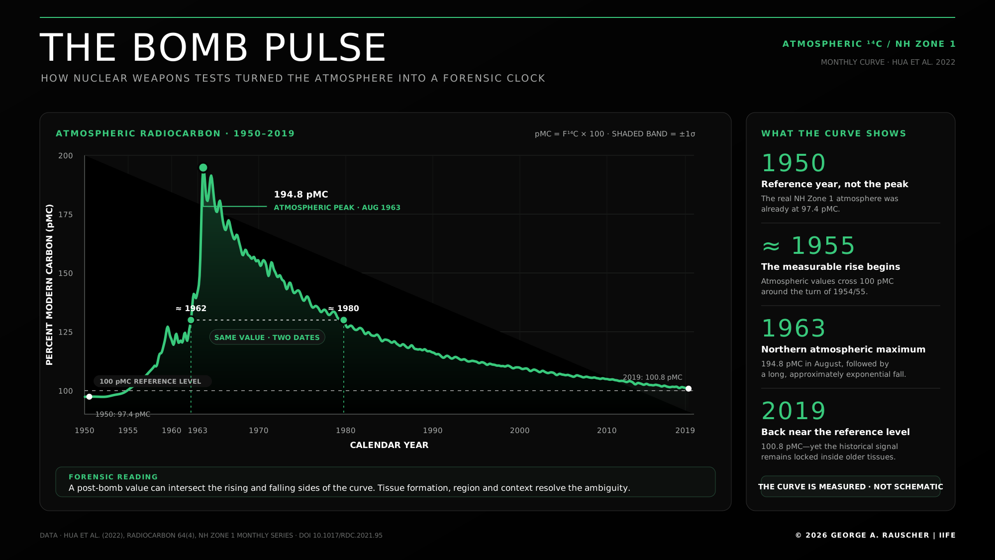
Atmospheric carbon-14 rose sharply after 1955 and reached 194.8 pMC in Northern Hemisphere Zone 1 in August 1963. It then declined approximately exponentially, returning to 100.8 pMC by 2019. Because the same post-bomb value can intersect the rising and falling sides of the curve, tissue type, region and biological context are essential for resolving the correct formation date. Data: Hua et al. (2022), monthly NH Zone 1 series.
From the early 1950s onward several nuclear powers conducted atmospheric weapons tests, in a number and explosive yield one can hardly picture today. The most intense series, the ones that shaped the bomb pulse, fell in the 1950s and early 1960s. These explosions released enormous quantities of neutrons, and neutrons in the atmosphere do what they always do: they strike nitrogen and produce carbon-14.
The result was a near doubling of the atmospheric C14 content compared with the preindustrial level, with the maximum in the year 1963 in the Northern Hemisphere. The Southern Hemisphere followed with a delay of one to 2 years, because the air masses of the hemispheres mix only slowly and the tests took place predominantly in the north. In 1963 the Partial Test Ban Treaty was signed. It ended atmospheric testing only for its parties at the time, individual states continued for more than a decade longer, and even so the atmospheric maximum in the Northern Hemisphere fell in 1963. Since then the curve has been falling again.
What matters is why it falls. Not through decay, for which the half-life is far too long. It falls because the excess carbon migrates out of the air into the oceans and the biosphere, and this exchange has a characteristic time constant of roughly 16 years. Ingeborg Levin and Bernd Kromer determined that from the measurement series at the Schauinsland in the Black Forest, one of the longest continuous atmospheric C14 time series in existence.
This gives us, for the period from 1955 onward, a steeply running curve on which individual years can be distinguished where the classical method can only separate centuries. The current reference datasets come from Quan Hua and colleagues and now cover the period 1950 to 2019, divided into 5 zones of atmospheric circulation, because the curve runs differently from region to region.
Kirsty Spalding, Bruce Buchholz, Henrik Druid and Jonas Frisén showed in Nature in 2005 what this means forensically. Because enamel is not remodeled after formation, it carries the atmospheric value of those childhood years in which the crown mineralized. Measure that value, compare it against the bomb curve and account for the known formation time of the particular tooth, and you have the year of birth. The authors state an accuracy of 1.6 years. For comparison they name in the same breath what classical morphological age estimation from skeleton and dental wear achieves in adults: 5 to 10 years.
Alongside that, the literature will show you a value of 1.0 plus minus 0.6 years, and that one comes from a later paper by Kanar Alkass and colleagues, published in 2010 in Molecular and Cellular Proteomics and based on 44 teeth from 41 individuals. There it stands beside a second figure that is every bit as interesting. The aspartic acid racemization carried out in parallel in dentine, which estimates actual age at death, came out at 5.4 plus minus 4.2 years. The 2 procedures correlated with a coefficient of determination of 0.66.
Why 2 different procedures at all? Because they answer different questions. The radiocarbon value in enamel says when someone was born. Racemization in dentine says how old someone became. From both together the year of death can be estimated with a quantifiable uncertainty, without needing a single document.
Eden Johnstone-Belford and Soren Blau reviewed the entire literature on bomb pulse dating of unidentified remains in 2020 and arrive at a two-sided conclusion. The results are reliable and accurate, but the studies so far rest predominantly on small samples and come almost exclusively from the Northern Hemisphere. And this is the point at which the method becomes invaluable for unidentified dead. A skeleton without papers, without clothing, without witnesses gives you an estimated sex, an estimated stature and a rough age range through anthropology. With that you search a missing persons database holding thousands of entries. Add a year of birth with 1 to 2 years of uncertainty, and the pool of matching missing person cases can shrink considerably while the investigation gains focus. In some cases that is the difference between an identification and a grave without a name.
The clock that is running out
And now the bad news, which barely features in public awareness at all.
The bomb pulse is disappearing from the atmosphere. It is not weakening in the sense of becoming blurrier, it is disappearing as a signal, because the curve is falling back to the natural level and within the foreseeable future below it, driven by the Suess effect, by our own fossil emissions. Heather Graven calculated this through in the Proceedings of the National Academy of Sciences in 2015, and the finding is uncomfortably clear: if we keep blowing fossil, C14-free carbon into the air, the atmosphere keeps aging in radiocarbon terms, and at some point fresh material yields values indistinguishable from old material.
For the dating of tissue formed in the coming years this means the bomb pulse method loses its uniqueness. For tooth enamel formed today or in the future, assignment through the bomb curve can become considerably more ambiguous and require additional information. How fast that happens depends on how fossil emissions develop.
Here I have to head off a misunderstanding I fell for myself. The bomb pulse signal in tissues formed during the past decades is preserved and will still be measurable in 50 years. Tooth enamel from 1970 carries its value from that time onward unchanged, entirely regardless of what today’s atmosphere does. For cold cases, therefore, no window is closing. What becomes harder is the assignment of tissue forming today and in the future, because its values increasingly overlap with preindustrial and older ranges. The tool is not vanishing from existing cases, it is losing its uniqueness for material formed from here on.
What the isotopes deliver along the way
If you are extracting collagen and measuring isotopes anyway, a whole set of information comes along almost as a byproduct, and with an unknown decedent that information is often worth more than the date itself.
Delta-13C separates food chains from one another. Plants with different photosynthetic pathways differ systematically. Most native European food plants belong to the C3 group, maize and millet to the C4 group. A high share of C4 plants such as maize or millet can show up in the carbon values, provided other food sources and local comparative values are taken into account.
Delta-15N rises with trophic level, with the share of animal protein, and it is elevated in breastfed infants, because the child stands, so to speak, one level above the mother. From incremental tooth sections one can reconstruct when a child was weaned. And, as I learned painfully above, it also rises with the aridity of the ecosystem, which is why it must never be interpreted on its own.
Sulfur, delta-34S, helps together with carbon and nitrogen to separate marine, terrestrial and in part freshwater food sources from one another. A standalone test for fish consumption it is not, but it was this combination that led Touzeau and colleagues to their finding.
Delta-18O in tooth enamel can give indications of drinking water, climate and mobility during tooth formation. Diet, physiology, breastfeeding and the preparation of food and water can, however, shift this signal.
And the strontium ratio of 87Sr to 86Sr is one of the most important geochemical markers for mobility and possible regions of upbringing. Strontium comes from the bedrock, travels through water and food into the body and is built into the calcium lattice of tooth enamel. Because this enamel is not remodeled afterward, it preserves the geological signal of the region in which someone grew up. Comparing tooth enamel and bone from the same person shows indications of whether the geochemical environment changed between childhood and later life. The bone value does not thereby designate the place of death, it reflects rather the residence and dietary context of the final years. A caveat belongs with this, and it grows more serious the more modern the case: in a world where food from every corner of the earth sits on the shelf, the provenance signal gets washed out. In premodern populations local food chains can often be delimited better than today. Even there the assignment remains probabilistic and depends on suitable local comparative data. For a missing person today it is an indication and not proof.
Taken together, suitably chosen tissues can yield indications of a birth range, a death range, a region of upbringing, a diet and migration, a biological profile of a person whose name nobody knows. That does, however, require several samples with different formation and turnover times, not a single one.
The leather belt, the ivory and the forged canvas
Up to here it has been about human beings. Datable, however, is everything that once took part in the carbon cycle, and that is quite a lot.
At an excavation somebody finds a leather belt. Leather is animal hide, animal hide is collagen, collagen is datable. The same holds for textiles of linen, wool or cotton, for wood and charcoal, parchment and paper, bone tools, food residues in a potsherd, seeds and grains. Not datable is the mineral matrix of metal, stone and ceramic, because there is no biogenic carbon in it. Organic tempering, food residues, soot and other carbon-bearing constituents within or upon them very much are. You do not date a bronze blade, you date the wood of its handle or the organic residues on it.
With ivory it becomes political. Kevin Uno and colleagues showed in the Proceedings of the National Academy of Sciences in 2013 that the bomb curve can determine when the sampled section of a tusk was formed, from which, with suitable and most recently formed substance, the animal’s time of death can be narrowed down closely. That makes it possible to distinguish whether a seized tusk comes from legal old stock or from a killing after the trade ban. Thure Cerling and colleagues continued this on seized material in 2016 and also determined the interval between death and seizure, which permits conclusions about smuggling routes. A method developed for archaeology now proves poaching.
With art it becomes entertaining. Anyone wanting to sell a painting as old needs an old canvas, and old canvases can be obtained. What is harder to fake are the organic binders. If the material contains carbon with a bomb pulse signature, then it grew after 1955, and the discussion about the supposed 18th century master is over before it begins. Laura Caforio and colleagues published this in 2014. I like this application in particular because it contains a fine reversal: of all things, the radioactive contamination of the atmosphere, the dirtiest legacy of the Cold War, is today one of the most effective means of refuting age claims about works of art. It can prove a forgery, but it cannot confirm authorship or provenance.
And then there is the industrial application that hardly anyone knows about, even though it runs daily. When a company claims its plastic is biobased, made from renewable raw materials rather than petroleum, that can be measured. Petroleum is C14-free, plant material is not. From the normalized share of modern carbon, the biobased carbon content is calculated under the standard ASTM D6866. A sustainability claim you do not have to believe but can count. There are fields where I would wish for that rather more often.
Whoever does not date is investigating blind
Now the part where I drop my restraint.
In the proceedings I have accompanied over the years, one pattern makes me less angry than tired. Proceedings are opened, apartments searched, collections seized, people entered as defendants, and in an alarming number of these cases the one examination that could objectively narrow the decisive period is never commissioned. People investigate the origin of bones for months without anybody having determined their age.
The laboratories exist, they work internationally, and the sample quantities are minimal. What is missing most often in my experience is not the budget but the knowledge that this possibility exists at all. You do not commission what you do not know about.
And that is why I am writing this text. Not as advertising, but because I believe an investigator who understands what a pMC value above 100 means makes better decisions than one who looks at a photograph and says it looks old. A skull that looks brand new can be millennia old. A skeleton that seems centuries old can date from the 1970s. With human remains, appearance is the least reliable witness there is, and yet in practice it decides whether proceedings are opened.
There is a boundary here that I want to name, because I do not want to cross it. Whether and how German courts assess radiocarbon findings in individual cases is something on which, after my research, I am aware of no published decision that treats the question in depth. What I can say is that the forensic literature measures the method against the usual standards of testability, standardized protocols, known error rates, validation through peer-reviewed publications and acceptance within the relevant scientific community, and holds it to be sound as a procedure. The evidentiary weight of an individual finding nonetheless depends on material selection, sample preparation, measurement uncertainty, calibration, reservoir and dietary effects and competent interpretation. That is a scientific statement and not a legal one. Anyone who needs a legal one has to obtain it from somebody trained for that.
What this method cannot do
So that we understand each other properly, here is the list of what you must not expect, in full sentences and without softening.
C14 does not date the moment of death but the end of carbon exchange, and depending on the tissue, years to decades lie between the two. C14 does not date the mineral fraction of rock, metal or ceramic, and it does not date fossils beyond 50,000 years, because either no biogenic carbon is present or the remaining share can no longer be reliably resolved against instrument background and contamination risk. Suitable organic residues on or within such objects very much are datable. C14 identifies no person, it only narrows a period, and identification requires DNA, dental status or other comparative features. C14 says nothing about cause of death. And C14 delivers no date but a distribution, as you saw with my 3 intervals.
Anyone who states these limits cleanly helps the proceedings. Anyone who conceals them and feigns certainty does more damage than someone who measured nothing at all, because a wrong number with a laboratory stamp is harder to get out of a case file than an honest gap in knowledge.
Back to the woods
The body in the jeans I began with can now be placed in a few steps with what you know.
You take several tissues with different formation and turnover times, never a single sample. Tooth enamel can narrow the year of birth through the bomb pulse, provided the dentition survives. Hair, nails or other rapidly turned over tissues sit closest in time to the death, provided they are still present and uncontaminated. Trabecula-rich bone rounds out the picture but, because of the delayed remodeling, likewise yields no precise year of death, only a signal averaged across years, and compact femoral shaft is particularly unfavorable for a dating as close to death as possible, because its collagen integrates a long period.
If a suitable tissue shows a pMC value clearly above 100, then it was formed after the start of the bomb pulse. That settles the possible medico-legal relevance, but not automatically a criminal offense, because the material may just as well come from a legal collection or a known burial. If the value does not lie significantly above 100, no simple separation between historical and modern follows from it alone, because since the 2020s freshly formed material itself falls below 100 again. Classical calibration, bomb pulse curves, possible reservoir corrections and further tissues then have to be evaluated together. If that yields a clearly historical period, it regularly changes the jurisdiction and the direction of the investigation, but it does not end it. Whether criminal, heritage, scientific, humanitarian or provenance questions remain open is decided independently of the mere age of the find.
All the rest of it is clean craft. Documentation of the discovery situation, careful removal without contamination, a note on every treatment the material has ever received, and a report that states the limits of the result as plainly as the result itself.
What came out in this particular case does not belong here. But I can tell you what it feels like when the numbers come back. It is a very quiet moment. There lies a sheet of paper on which a human being has been reduced to a ratio of isotopes, and this ratio decides whether a family gets an answer after decades or whether a file number is closed. In this profession I have learned to phrase findings coldly. That one moment refuses to stay cold.
Too expensive, too rarely used, and I have nothing better to offer
With that we are back at the point I announced at the beginning, and it is the only one where I cannot end this text coldly.
We have a method that has worked for more than 75 years, that operates on almost every organic material, that reaches back roughly 50,000 years, whose error margins are known and published, and that answers a question on which entire investigations hang. And it is used far too rarely. Bertrand and colleagues wrote it out openly in 2024, that the method is still underused in forensic anthropology, and they name as reasons cost and turnaround time, which practitioners regularly overestimate. That matches my experience, and technical doubt it certainly is not. A dating costs money, an accelerator costs millions, a laboratory costs continuously, and on top of that come institutional workflows and simply missing knowledge of what is possible. Somewhere in this chain sits a person who administers a budget and decides that one can manage without.
One cannot in fact manage without it. One merely investigates as though one could, and that is a difference you notice only when the result exonerates or incriminates somebody years later who was in the wrong drawer the whole time.
It would therefore be time to look seriously for alternatives, for procedures that answer the same question more cheaply. And here I have to be honest, because I have no equivalent replacement to offer. There are cheaper procedures that can pre-sort or supplement, such as aspartic acid racemization in dentine, which I described further above, along with histological and spectroscopic methods. A partner procedure is not a replacement, however, because racemization estimates age at death and not the point in time. A universal substitute that delivers the same direct isotopic chronology across this range of materials and periods is not known to me. So I am putting the task here without being able to solve it, and I consider that the more honest option than pretending I have an idea in a drawer.
What remains until then is the method itself, correctly applied. Anyone who finds human remains calls the police and takes no samples, because improper removal destroys a result before it exists. Anyone dealing with such a find as an investigator or an expert asks the question of the period first and all others afterward. And anyone handed a certificate reads it the way I have read one to you here, with the pMC value, the formula, the calibrated ranges and the line about what was not calculated.
A tooth from Thebes, measured with an instrument that counts individual atoms, yields 3 time windows, a high nitrogen value that in the Egyptian comparison is more consistent with dryness than with regular fish consumption, and a time window that possibly reflects predominantly this woman’s tooth formation phase and in any case not her death. None of that is a shortcoming of the method. It is the method, read honestly.
And if you take a single sentence away from this entire text, take this one: with every dating result somebody puts in front of you, ask which tissue was measured. The answer to that one question decides the correctness of a finding more often than the whole remaining discussion around it.
Nothing more from me on this subject, and I hope it has come a little closer to you.
This article complements the older text on C14 analysis of human remains on rauscher.xyz and develops its subject in technical depth. Editorial status: July 31, 2026.
References
- Alkass, K., Buchholz, B. A., Ohtani, S., Yamamoto, T., Druid, H., & Spalding, K. L. (2010). Age estimation in forensic sciences: Application of combined aspartic acid racemization and radiocarbon analysis. Molecular & Cellular Proteomics, 9(5), 1022 to 1030. https://doi.org/10.1074/mcp.M900525-MCP200
- AlQahtani, S. J., Hector, M. P., & Liversidge, H. M. (2010). Brief communication: The London atlas of human tooth development and eruption. American Journal of Physical Anthropology, 142(3), 481 to 490. https://doi.org/10.1002/ajpa.21258
- Ambrose, S. H. (1990). Preparation and characterization of bone and tooth collagen for isotopic analysis. Journal of Archaeological Science, 17(4), 431 to 451.
- Anonymized AMS laboratory report on sample „Female mummy 215, Thebes 1877″, internal identifier Sample A, unpublished, author’s archive.
- Barlovic, I. (2015, December 8). C-14 Labor Erlangen wurde geschlossen. about-africa.de. https://www.about-africa.de/diverses-unsortiertes/631-c-14-labor-erlangen-wurde-geschlossen
- Bertrand, B., Clauzel, T., Richardin, P., Bécart, A., Morbidelli, P., Hédouin, V., & Marques, C. (2024). Application and implications of radiocarbon dating in forensic case work: When medico-legal significance meets archaeological relevance. Forensic Sciences Research, 9(3), owae046. https://doi.org/10.1093/fsr/owae046
- Bronk Ramsey, C. (2009). Bayesian analysis of radiocarbon dates. Radiocarbon, 51(1), 337 to 360. https://doi.org/10.1017/S0033822200033865
- Caforio, L., Fedi, M. E., Mandò, P. A., Minarelli, F., Peccenini, E., Pellicori, V., Petrucci, F. C., Schwartzbaum, P., & Taccetti, F. (2014). Discovering forgeries of modern art by the 14C bomb peak. European Physical Journal Plus, 129, 6. https://doi.org/10.1140/epjp/i2014-14006-6
- Cerling, T. E., Barnette, J. E., Chesson, L. A., Douglas-Hamilton, I., Gobush, K. S., Uno, K. T., Wasser, S. K., & Xu, X. (2016). Radiocarbon dating of seized ivory confirms rapid decline in African elephant populations and provides insight into illegal trade. Proceedings of the National Academy of Sciences, 113(47), 13330 to 13335. https://doi.org/10.1073/pnas.1614938113
- Cook, G. T., Bonsall, C., Hedges, R. E. M., McSweeney, K., Boroneanţ, V., & Pettitt, P. B. (2001). A freshwater diet-derived 14C reservoir effect at the Stone Age sites in the Iron Gates Gorge. Radiocarbon, 43(2A), 453 to 460.
- Czermak, A., Fernández-Crespo, T., Ditchfield, P. W., & Lee-Thorp, J. A. (2020). A guide for an anatomically sensitive dentine microsampling and age-alignment approach for human teeth isotopic sequences. American Journal of Physical Anthropology, 173(4), 776 to 783. https://doi.org/10.1002/ajpa.24126
- DeNiro, M. J. (1985). Postmortem preservation and alteration of in vivo bone collagen isotope ratios in relation to palaeodietary reconstruction. Nature, 317, 806 to 809. https://doi.org/10.1038/317806a0
- Freeman, S., Bishop, P., Bryant, C., Cook, G., Fallick, A., Harkness, D., Metcalfe, S., Scott, M., Scott, R., & Summerfield, M. (2004). A new environmental sciences AMS laboratory in Scotland. Nuclear Instruments and Methods in Physics Research B, 223 to 224, 195 to 198.
- Godwin, H. (1962). Half-life of radiocarbon. Nature, 195, 984. https://doi.org/10.1038/195984a0
- Graven, H. D. (2015). Impact of fossil fuel emissions on atmospheric radiocarbon and various applications of radiocarbon over this century. Proceedings of the National Academy of Sciences, 112(31), 9542 to 9545. https://doi.org/10.1073/pnas.1504467112
- Heaton, T. J., Blaauw, M., Blackwell, P. G., Bronk Ramsey, C., Reimer, P. J., & Scott, E. M. (2020). The IntCal20 approach to radiocarbon calibration curve construction: A new methodology using Bayesian splines and errors-in-variables. Radiocarbon, 62(4), 821 to 863. https://doi.org/10.1017/RDC.2020.46
- Heaton, T. J., Köhler, P., Butzin, M., Bard, E., Reimer, R. W., Austin, W. E. N., Bronk Ramsey, C., Grootes, P. M., Hughen, K. A., Kromer, B., Reimer, P. J., Adkins, J., Burke, A., Cook, M. S., Olsen, J., & Skinner, L. C. (2020). Marine20, the marine radiocarbon age calibration curve (0 to 55,000 cal BP). Radiocarbon, 62(4), 779 to 820. https://doi.org/10.1017/RDC.2020.68
- Hedges, R. E. M., Clement, J. G., Thomas, C. D. L., & O’Connell, T. C. (2007). Collagen turnover in the adult femoral mid-shaft: Modeled from anthropogenic radiocarbon tracer measurements. American Journal of Physical Anthropology, 133(2), 808 to 816. https://doi.org/10.1002/ajpa.20598
- Hogg, A. G., Heaton, T. J., Hua, Q., Palmer, J. G., Turney, C. S. M., Southon, J., Bayliss, A., Blackwell, P. G., Boswijk, G., Bronk Ramsey, C., Pearson, C., Petchey, F., Reimer, P., Reimer, R., & Wacker, L. (2020). SHCal20 Southern Hemisphere calibration, 0 to 55,000 years cal BP. Radiocarbon, 62(4), 759 to 778. https://doi.org/10.1017/RDC.2020.59
- Hua, Q., Turnbull, J. C., Santos, G. M., Rakowski, A. Z., Ancapichún, S., De Pol-Holz, R., Hammer, S., Lehman, S. J., Levin, I., Miller, J. B., Palmer, J. G., & Turney, C. S. M. (2022). Atmospheric radiocarbon for the period 1950 to 2019. Radiocarbon, 64(4), 723 to 745. https://doi.org/10.1017/RDC.2021.95
- MICADAS, technical specification (compact radiocarbon AMS system).
- Johnstone-Belford, E. C., & Blau, S. (2020). A review of bomb pulse dating and its use in the investigation of unidentified human remains. Journal of Forensic Sciences, 65(3), 676 to 685. https://doi.org/10.1111/1556-4029.14227
- Kieser, W. E., Zhao, X.-L., Clark, I. D., Cornett, R. J., Litherland, A. E., Klein, M., Mous, D. J. W., & Alary, J.-F. (2015). The André E. Lalonde AMS Laboratory: The new accelerator mass spectrometry facility at the University of Ottawa. Nuclear Instruments and Methods in Physics Research B, 361, 110 to 114. https://doi.org/10.1016/j.nimb.2015.03.014
- Levin, I., & Kromer, B. (1997). Twenty years of atmospheric 14CO2 observations at Schauinsland station, Germany. Radiocarbon, 39(2), 205 to 218.
- Libby, W. F., Anderson, E. C., & Arnold, J. R. (1949). Age determination by radiocarbon content: World-wide assay of natural radiocarbon. Science, 109(2827), 227 to 228. https://doi.org/10.1126/science.109.2827.227
- Lynnerup, N., Kjeldsen, H., Heegaard, S., Jacobsen, C., & Heinemeier, J. (2008). Radiocarbon dating of the human eye lens crystallines reveal proteins without carbon turnover throughout life. PLoS ONE, 3(1), e1529. https://doi.org/10.1371/journal.pone.0001529
- National Science Foundation. (1998). Major Research Instrumentation Program, 1998 MRI awards, award 9871035. https://www.nsf.gov/od/oia/programs/mri/1998.jsp
- Philippsen, B. (2013). The freshwater reservoir effect in radiocarbon dating. Heritage Science, 1, 24. https://doi.org/10.1186/2050-7445-1-24
- Ravi Prasad, G. V., Noakes, J. E., Cherkinsky, A., Culp, R., & Dvoracek, D. (2013). The new 250 kV single stage AMS system at CAIS, University of Georgia: Performance comparison with a 500 kV compact tandem machine. Radiocarbon, 55(2 to 3), 319 to 324.
- Reimer, P. J., Austin, W. E. N., Bard, E., Bayliss, A., Blackwell, P. G., Bronk Ramsey, C., Butzin, M., Cheng, H., Edwards, R. L., Friedrich, M., Grootes, P. M., Guilderson, T. P., Hajdas, I., Heaton, T. J., Hogg, A. G., Hughen, K. A., Kromer, B., Manning, S. W., Muscheler, R., … Talamo, S. (2020). The IntCal20 Northern Hemisphere radiocarbon age calibration curve (0 to 55 cal kBP). Radiocarbon, 62(4), 725 to 757. https://doi.org/10.1017/RDC.2020.41
- Spalding, K. L., Buchholz, B. A., Bergman, L.-E., Druid, H., & Frisén, J. (2005). Forensics: Age written in teeth by nuclear tests. Nature, 437(7057), 333 to 334. https://doi.org/10.1038/437333a
- Strafgesetzbuch (StGB), Section 78 subsection 2, limitation period. Bundesministerium der Justiz. https://www.gesetze-im-internet.de/stgb/__78.html
- Stuiver, M., & Polach, H. A. (1977). Discussion: Reporting of 14C data. Radiocarbon, 19(3), 355 to 363. https://doi.org/10.1017/S0033822200003672
- Synal, H.-A., Stocker, M., & Suter, M. (2007). MICADAS: A new compact radiocarbon AMS system. Nuclear Instruments and Methods in Physics Research B, 259(1), 7 to 13. https://doi.org/10.1016/j.nimb.2007.01.138
- Touzeau, A., Amiot, R., Blichert-Toft, J., Flandrois, J.-P., Fourel, F., Grossi, V., Martineau, F., Richardin, P., & Lécuyer, C. (2014). Diet of ancient Egyptians inferred from stable isotope systematics. Journal of Archaeological Science, 46, 114 to 124. https://doi.org/10.1016/j.jas.2014.03.005
- Ubelaker, D. H. (2014). Radiocarbon analysis of human remains: A review of forensic applications. Journal of Forensic Sciences, 59(6), 1466 to 1472. https://doi.org/10.1111/1556-4029.12535
- Ubelaker, D. H., Buchholz, B. A., & Stewart, J. E. B. (2006). Analysis of artificial radiocarbon in different skeletal and dental tissue types to evaluate date of death. Journal of Forensic Sciences, 51(3), 484 to 488. https://doi.org/10.1111/j.1556-4029.2006.00125.x
- Uno, K. T., Quade, J., Fisher, D. C., Wittemyer, G., Douglas-Hamilton, I., Andanje, S., Omondi, P., Litoroh, M., & Cerling, T. E. (2013). Bomb-curve radiocarbon measurement of recent biologic tissues and applications to wildlife forensics and stable isotope (paleo)ecology. Proceedings of the National Academy of Sciences, 110(29), 11736 to 11741. https://doi.org/10.1073/pnas.1302226110
- Völkerstrafgesetzbuch (VStGB), Section 5, non-applicability of limitation. Bundesministerium der Justiz. https://www.gesetze-im-internet.de/vstgb/__5.html
Keywords: What is radiocarbon dating, radiocarbon dating, carbon-14 dating, C14 dating, carbon-14 half-life, bone age determination, bomb pulse, IntCal20 calibration curve, tooth enamel year of birth, forensic anthropology
Disclaimer: This article reflects the author’s own research and opinion as of the publication date shown above; later findings or legal changes may have overtaken it, so always check that date. Sources are cited for independent verification, and no liability is accepted for third-party studies. This is general information, not medical, legal, or professional advice: for medical questions see a doctor, for legal questions a lawyer, and in an acute crisis contact emergency services or a crisis helpline.
About the header image: it is AI-generated. Cheaper than a photo shoot, and I have made my peace with the age of AI. Everything inside the article is real, the diagrams, the skulls, the findings, and every word. The machine gets the opening shot and not one inch past it.

Is It Legal to Own a Real Human Skull? Yes, Subject to 3 Conditions
Private possession of a real human skull is not prohibited in Germany. Three conditions decide the question, and…

The Science and Ethics of Age-Gap Attraction: Why Older Men Are Drawn to Younger Women, and Where the Line to Crime Runs
A forensic examiner lays out the evolutionary psychology and the data from 130 countries: the algorithm of age-gap…
The Pressure Fallacy: What Pink Teeth in the Dead Really Reveal, and What They Do Not
A forensic investigation through 200 years of literature, prompted by three cases, two of which I examined myself,…